The IMADA DST series digital force gauge ships with Force Logger communication software that transfers readings to a PC, calculates maximum / minimum / average values and exports CSV. But as soon as the test object changes from "reading a number" to "observing a process", the bundled software is no longer enough — it logs discrete points and has no force curve.
In tests such as insertion/extraction force, button feel and spring stiffness, the real information lies in the shape of the curve: slope, inflection points, plateaus, jitter and rebound. Two presses can both peak at 12.20 N — one a clean bottom-out, the other a stick-then-snap — and the numbers alone cannot tell them apart. We therefore developed companion PC software that retains the original numerical logging and adds a live force curve, multi-curve overlay comparison, and triggered / timed automatic recording. This article explains the technical background and how to use it.
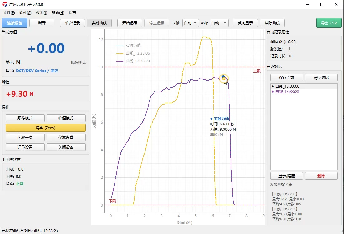
Figure 1 Two measured curves overlaid: yellow is the 12.20 N peak curve, purple the 9.30 N curve, dashed lines are the configured upper and lower limits
I. Why the bundled Force Logger is not enough
According to IMADA's official documentation, the bundled Force Logger for the DST / DSV series is positioned as peak data acquisition: it reads measured values, calculates maximum / minimum / average, and saves them as CSV at roughly 10 points per second. It can answer "how much was measured", but not "how the force was applied".
IMADA also offers the SW-1X data acquisition software, which can generate a profile graph, but it is an optional extra, not part of the standard bundle. For production stations that only need single-point pass/fail judgement, the bundled software is adequate; for process analysis, failure reproduction or customer reports, the missing piece is a curve.
Our software fills exactly this gap: it does not change the instrument's accuracy or judgement logic; it simply takes the data the gauge already outputs over the serial port and plots, stores and overlays it at a higher time resolution.
II. Communication basics of the DST series
2.1 Two physical interfaces, the same serial semantics
- USB: enumerated as a virtual COM port, 8 data bits, 1 stop bit, no parity (8-N-1), baud rate 256000; it also handles charging and can be powered from a PC USB port or a power bank.
- RS-232C: 8-N-1 at 19200 baud, suitable for connection to industrial PCs, PLCs or older data acquisition equipment.
- Capacity and accuracy: the DST series covers 2 N / 5 N / 20 N / 50 N / 200 N / 500 N / 1000 N, with accuracy ±0.2% F.S. ±1 digit, overload capacity about 200% F.S., warning from 90% of range and a flashing display from 110%.
2.2 Sampling rate ≠ output rate
This is the point most often misunderstood during selection. The instrument's internal sampling rate is very high — IMADA specifies 30,000 samples per second (some regional literature quotes a measurement frequency of 1000 per second) — to catch the instantaneous peak in a destructive test; but the rate at which data reaches the PC is set by the communication cycle, and the bundled Force Logger logs at about 10 points per second.
In other words, the peak shown on the gauge display is reliable, but whether the curve on your PC "keeps up" depends on the interval at which the software polls. Our software brings the minimum logging interval down to 0.05 s (20 points per second), twice that of the bundled software — enough to reconstruct the outline of millisecond-scale transitions such as button actuation or terminal pull-off. Note: the outline, not the raw samples. To capture true transient spikes, still rely on the instrument's own peak hold; the software-side curve is for seeing process shape.
2.3 Two engineering issues the software must handle
- Timestamps must not be derived from "point count × interval".A serial port drops frames when the system is busy; accumulating time by point count drifts the entire X axis and two curves will never line up again. Time must be stamped locally at the moment each frame is received.
- Acquisition and drawing must be decoupled.If every incoming frame triggers a redraw, dragging the window or switching tabs blocks serial reads and the curve shows cliff-like gaps. The interface must remain usable and the curve continuous during logging — a basic test of whether acquisition software is fit for purpose.
One more reminder: moving a USB virtual COM port to a different USB socket usually changes the port number (COM3 becomes COM5). The software shows a model hint based on the port name, but that is only a hint; the model shown on the gauge display is authoritative — DST gauges of different capacities look almost identical, and connecting the wrong capacity is far more serious than choosing the wrong port.
III. Feature comparison: manufacturer software vs companion software
| Feature | Force Logger (bundled) | Yunke companion software |
| Live value / peak display | Supported | Supported (track / peak mode switch) |
| Max / min / average statistics | Supported | Supported (includes point count) |
| CSV export | Supported | Supported |
| Instrument parameter setup | Supported | Supported (limits, unit system, display direction) |
| Live force curve | — | Supported, 0.05 s minimum interval |
| Multi-curve overlay comparison | — | Supported, multiple curves on screen |
| Graphical upper/lower limit lines | Numeric judgement only | Upper / lower limits marked directly on the curve |
| Triggered / timed recording | — | Supported, configurable trigger value |
| Y axis / X axis range | — | Switchable auto / manual |
| Curve cursor readout | — | Supported, shows time and force |
The Force Logger column follows IMADA's official and authorised-channel published feature descriptions; that software remains in the standard accessory kit, and ours is a complement, not a replacement.
IV. Feature walkthrough
The screen recording below shows the complete workflow on a DST series sample unit, from connecting the device and live logging to saving curves for comparison, about two minutes:
Video DST series live session: connect → zero → live logging → curve comparison → export
4.1 Connection and device status
Select the serial port and click "Connect"; the status bar shows a line of diagnostics: device model, identification source and raw response. Model identification first uses the instrument's self-reported information, falling back to a port-name hint. The "raw response" is for troubleshooting communication failures — check this line first when you cannot connect; it is more effective than repeatedly unplugging the cable.
The left panel also shows current force and peak, with units following the instrument's unit setting (N / kg / Lb). Limit status is given directly as "Normal / Over upper / Under lower", consistent with the gauge's own comparator judgement.
4.2 Live curve
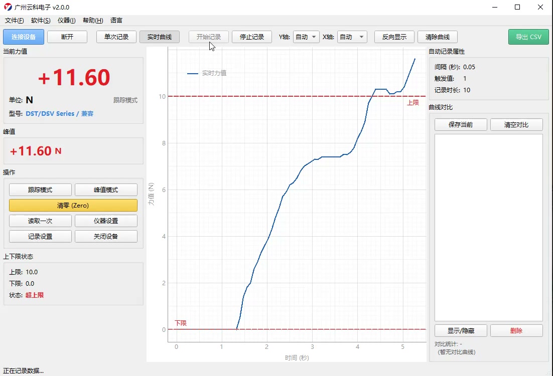
Figure 2 During live logging: the rising segment is clearly visible and the status changes to "Over upper" when force crosses the upper limit
Click the "Live Curve" tab to enter plotting mode; the vertical axis is force (N) and the horizontal axis is time (s). Three dashed lines mark the configured upper limit, lower limit and zero reference. On a limit breach the curve and the status both turn red, so you can see at a glance that the press went too far without watching the numbers.
- Y axis / X axis: auto range by default, so the curve rescales with the force range; switch to manual for repeatability comparisons, where multiple curves must share exactly the same coordinates.
- Reverse display: matches the reading convention for tension tests (display direction opposite to compression), avoiding negative values in reports.
- Cursor: hover over the curve to show time and force at that point, for locating inflection points or reading the average of a plateau.
4.3 Automatic logging: trigger and timer
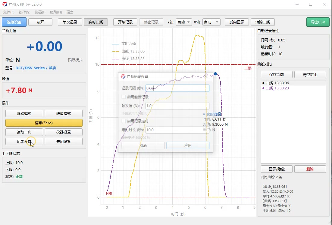
Figure 3 Automatic logging setup: interval 0.05 s, trigger value 1.0 N, timer 10 s
Clicking "Start Logging" manually suits a single test; for batch testing use automatic logging. The two trigger modes can be combined:
- Triggered logging: recording starts only when force exceeds a configured threshold (e.g. 1.0 N), so unloaded noise near zero is kept out of the curve and each test produces a more consistent data length.
- Timed logging: stops automatically at a set time, suitable for tests with a duration requirement such as "press for 10 s to observe creep". The interface supports up to 60,000 s, enough for long hold tests.
At a 0.05 s logging interval you get 20 points per second. Shorter intervals give finer curves but larger data volumes — 0.05 s is sufficient for a 2 s button test; for a 10-minute creep test, widen it to 0.2–0.5 s or the CSV becomes unwieldy.
4.4 Curve comparison: the core of our development
After a test, click "Save Current" and the curve enters the comparison list on the right, where it can be named, shown/hidden or deleted. Run a second test and the two curves appear in the same coordinate system, making differences obvious.
The lower right shows statistics for each curve: maximum, minimum, average and point count. For batch consistency checks there is no need to export CSV and plot in Excel — just change the workpiece, measure again and compare in the software.
Three typical uses:
- First-piece vs last-piece comparison: record a baseline curve at the start of a shift on a station, then measure one more piece before the end of the shift and overlay it; a changed shape points to a loose fixture or a change in workpiece batch.
- Defect reproduction: overlay a customer-returned failed part with a good part; the moment at which sticking or a second peak appears is far more intuitive than a written description.
- Process parameter validation: after changing a spring, lubricant or press-fit speed, save one curve per condition; changes in slope and peak are the effect of the process change.
4.5 Logged data and export
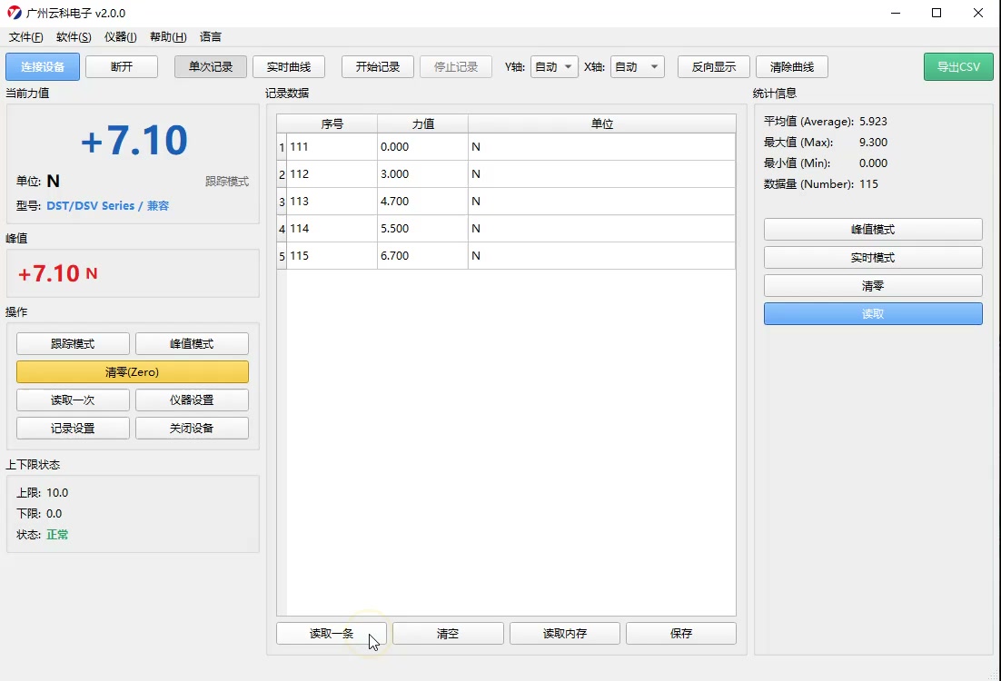
Figure 4 Logged data tab: point-by-point table plus average / maximum / minimum / data count
The "Logged Data" tab reconstructs the current curve as a point-by-point table (index, force, unit), with statistics shown alongside. Four buttons at the bottom correspond to different sources: read one (current gauge value), read memory (gauge internal storage, DSV series supports 1000 sets), clear and save.
For reports or further analysis, click "Export CSV". The file is standard comma-separated text readable directly by Excel, Origin and Python, with columns identical to the on-screen table and no extra processing — avoiding disputes where "the software shows one value and the export shows another".
The "File" menu also offers "Save to Database" and "History Management" for keeping local test records searchable by time, without hunting through folders for CSV files each time.
V. Three typical scenarios
5.1 Button / switch feel
Feel comes down to the "actuation point" and "rebound": the slope of the rising segment reflects how quickly force builds, the first peak is the actuation force, the drop after the peak is the travel feel, and the step on release is the return force. Good switches of the same model have highly consistent curve shapes; a double peak or a collapsed plateau almost always means an internal spring contact or assembly problem. Judgements like this cannot be made from numbers, but are obvious from a curve.
5.2 Connector insertion / extraction force
Insertion usually has three phases: lead-in (alignment), ramp-up (terminal contact) and hold (fully seated). National and in-house standards often specify insertion peak and extraction force separately; looking at a single peak misses hidden defects such as "sticking during insertion" — the sawtooth on the curve is the sticking. Overlay a good and a bad part and you can read directly where in the travel it stuck and how much force was involved.
5.3 Spring force / stiffness
When compressing a spring, the force–displacement curve is approximately a straight line whose slope is the stiffness. DST outputs a force–time curve; under constant-speed compression the time axis is equivalent to a displacement axis, so a change in slope is a change in stiffness. For batch sampling of springs, keep the first-piece curve as a baseline and overlay each subsequent piece; a slope deviation beyond an agreed proportion is flagged as abnormal, which is better at finding wrong coil counts or soft material than a single-point force check.
VI. Workflow (from wiring to report)
- Wiring: connect the gauge to the PC with a USB cable and install the virtual COM driver on first use; with RS-232C, confirm crossover/straight-through wiring and the 19200 baud rate.
- Fit the fixture: select hook, flat, conical or other attachments according to the sample, and hand-tighten onto the M6 measuring shaft; do not use a spanner.
- Zero: with no load, click "Zero" to remove attachment weight; re-zero after changing attachments or mounting orientation.
- Select mode: use "Track mode" to observe a process, "Peak mode" when only the peak is needed.
- Set judgement: enter upper/lower limits (Value1 / Value2) in "Instrument Settings" and click "Apply to Device"; the judgement logic resides in the gauge and is not lost when you change PCs.
- Record: click "Start Logging" for a single test; for batches use trigger / timer in "Logging Setup".
- Compare: after measuring, click "Save Current" and overlay with the baseline curve to check shape and statistics.
- Export: click "Export CSV", or "Save to Database" for archiving.
VII. Frequently asked questions
Cannot connect to the device?
Check the "raw response" in the status bar first: empty means the port did not open (occupied by other software, wrong port number, driver not installed); garbled text means the baud rate or data bits are wrong. With RS-232C also verify the wiring. Changing USB sockets changes the port number — this is the most common cause.
Are sawtooth patterns or gaps in the curve normal?
Sawtooth usually comes from a polling interval out of sync with the gauge's output cycle; setting the logging interval above 0.1 s normally improves it noticeably. Gaps are dropped frames — check whether the USB cable is too long, whether it passes through an unpowered hub, and whether the PC is running heavy tasks.
Software reading differs from the gauge display by 0.01?
Usually this is a difference in displayed digits and rounding. The software keeps more digits from the received raw value, while the gauge display rounds to its own resolution. The gauge setting is authoritative; the software applies no secondary correction.
Does the software affect instrument accuracy?
No. It only reads data the gauge has already output and takes no part in measurement or calibration. Accuracy remains ±0.2% F.S. ±1 digit, and calibration intervals and metrology requirements are unchanged whether or not the gauge is connected.
Which models are supported?
All DST and DSV models with USB or RS-232C output. The difference between the two series is features: DSV adds tilt alarms (4° / 8° / 18° sensitivity levels), continuous peak mode and 1000-set internal storage; communication interface and data output are identical.
VIII. Availability and adaptation
The Force Logger and USB cable in the original DST packaging remain unchanged; the companion software is supplied on request and supports all DST / DSV models with a communication interface. If you need to feed curves into an existing MES, add custom fields or export in bulk, contact us with your data format and workflow requirements.
DST series models available on this site: DST-500N、DST-200N、DST-50N、DST-20N. For selection and operating details see IMADA Force Gauge Operating Guide。
Note: the screenshots and screen recordings in this article were taken from the live interface of Guangzhou Yunke Electronics' in-house companion software v2.0.0; instrument specifications are quoted from IMADA official literature, and software features are subject to the delivered version.